Truncation Errors

Truncation Errors

Truncation Errors

Applying a finite difference operator has the side effect of introducing truncation errors into the solution. In this section we discuss how truncation enters the system and how it affects it.

Truncation and Dispersion^3.5
Consequences and Interpretation

Truncation and Dispersion

Earlier we presented a generic equation describing the conservation laws. This allows us to extract information of the numeric properties of the system quite easily, as the analysis of the one generic equation can be propagated to all its special cases. We will not make any assumptions on the drains and sources in the system, and hence do not include any such in this presentation, instead we consider the simple conserved system:

$\begin{displaymath}\frac{\partial \Gamma }{\partial t}=-\nabla \cdot \Gamma \mathbf{u}.\end{displaymath}$

Now, to make the analysis easier we initially consider the one dimensional case with constant velocity u,

$\begin{displaymath}\frac{\partial \Gamma }{\partial t}+u\frac{\partial \Gamma }{\partial x}=0.\end{displaymath}$

In a previous section we discussed the type and order of the difference operators, in the following we will limit the analysis to a simple centered difference operator, but as we will see the analysis is straight-forward, and may be performed using operators of any order. In continuous time, discrete space, with $\Gamma _{i}$ designating $\Gamma$ evaluated at grid node i, we find

$\begin{displaymath}\frac{\partial \Gamma }{\partial t}+u\frac{\Gamma _{i+1}-\Gamma _{i-1}}{2\Delta x}=0.\end{displaymath}$

As we have noted earlier, this discretisation implies losing some higher-order terms. To see why this happens we will express the above approximation by the Taylor expansion of the terms involved, as we approximate $\Gamma _{i+1}$ and $\Gamma _{i-1}$ by respectively expanding forward and backward from the value $\Gamma _{i}$ by the distance $\Delta x$ between any two grid nodes:

$\begin{eqnarray*}\Gamma _{i+1} & = & \Gamma _{i}+\frac{\Delta x}{1!}\frac{\parti... ...}\frac{\partial ^{3}\Gamma _{i}}{\partial x^{3}}+O(\Delta x^{5}) \end{eqnarray*}$

By inserting into the continuous time, discrete space approximation we find the equation we are actually solving

$\begin{displaymath}\frac{\partial \Gamma }{\partial t}+u\left( \frac{\partial \G... ...ial ^{3}\Gamma _{i}}{\partial x^{3}}+O(\Delta x^{4})\right) =0.\end{displaymath}$

Consequences and Interpretation

To give an impression of what this means for the solution, we now let $\Gamma$ represent a simple sinusoidal wave in time and space. We then isolate the temporal frequency and calculate the wave speed, from which we can gain some insight into how the system evolves. The wave can be described as $\Gamma =e^{ikx-i\omega t}$ which enables us to extend the argument, at least to periodic solutions as we simply approximate the shape through Fourier series. By simple insertion we find

$\begin{eqnarray*}& \frac{\partial \Gamma }{\partial t}+u\left( \frac{\partial \G... ...^{2}}{3!}k^{2}+...+(-1)^{n}\frac{\Delta x^{n}}{n!}k^{n}+...). & \end{eqnarray*}$

With spatial wave length $l=\frac{2\pi }{k}$ and time frequency $T=\frac{2\pi }{\omega }$ we find the wave speed

$\begin{displaymath}s=\frac{l}{T}=\frac{\omega }{k}=u(1-\frac{(k\Delta x)^{2}}{3!}...+(-1)^{n}\frac{(k\Delta x)^{n}}{n!}+...),\end{displaymath}$

which converges as the faculty operator is stronger than the power. We see that the speed at which a solution propagates is dependent on the spatial frequency, and that the most significant term enters with a negative coefficient, causing a slow down of frequencies. At constant grid spacing $\Delta x$ , and as a low value of k models a high spatial frequency wave, we can now see high frequency modes will move slower than low frequency ones. This means that over time a solution consisting of a broad range of frequencies will change shape, as high mode frequencies will be left behind. This is especially evident in the solution of the square wave, which has non-vanishing amplitude in all frequency modes, and hence all terms in the Taylor expansion are of importance. This is the origin of the dispersion phenomena mentioned in an earlier section. In our case this is especially worrying, as we have already seen, shocks may evolve naturally in the system, and hence the near discontinuities in the shock fronts result in high order frequencies dominating the system. This can be seen in figure 3.5

Figure 3.5: Constant velocity propagation of a steep wave using a naive implementation of the difference operator.

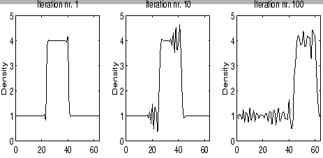
$\resizebox*{0.8\textwidth}{0.2\textheight}{\includegraphics{nodiff.eps}}$

, where we see how such a system evolves. We see that the truncation results in dispersion as high frequency modes are left behind by the bulk of the wave causing numerical instability due to the steep gradients flooding the solution. At roughly iteration number 130 the valley immediately following the hill became negative, crashing the simulation. As a rule of thumb truncation is of no immediate concern if the shock is resolved on the grid, i.e. the wave length of the highest mode frequency in the shock is a number of times longer than the grid spacing $\Delta x$ , as is also hinted by the term $k\Delta x$ entering under the power operator.

Another view at the problem is noticing that in the difference operation of order n we truncated

$\begin{displaymath}\frac{\Delta x^{n}}{n!}\frac{\partial ^{n}\Gamma _{i}}{\partial x^{n}}\end{displaymath}$

terms from the Taylor series from the order n and up, terms for which the coefficients $\Delta x^{n}/n!$ was in some sense small, under the assumption that the differential operator $\partial ^{n}\Gamma _{i}/\partial x^{n}$ is in some sense limited, making all the truncated terms insignificant for the solution. But at near discontinuities this is not the case, as $\partial ^{n}\Gamma _{i}/\partial x^{n}$ becomes of significance, breaking the assumption and infecting the solution.

The net result is that the truncation error will be of relevance in shock regions, and that we cannot approximate the solution correctly in an extreme shock-region, no matter the order of the difference operator. If ignored this will in many cases cause the discrete approximations to explode, and in return drown the correct solution in numerical noise.

But what if we could avoid the discontinuities altogether?